Transfer Learning for Image Recognition and Natural Language Processing

If you had the chance to read Part 1 of this article, you will remember that Transfer Learning is a machine learning method where the application of knowledge obtained from a model used in one task, can be reused as a foundation point for another task.

If you did not get the chance and don’t have a great understanding of Transfer Learning, give it a read it will help you understand this article much better. 

Image Recognition

 
So let's first go through what Image Recognition is. Image Recognition is the task assigned to computer technology to be able to detect and analyse an object or a feature in an image or video. It is the major area where deep neural networks work their magic as they are designed to recognise patterns. 

If you would like to see how neural networks analyse and grasp their understanding of images, take a look here. This shows you how lower-level layers concentrate on learning low-level features and how the higher-level layers adapt to learn higher-level features.

We vaguely spoke about training the network on cats and dogs in part 1 of this article, let's speak more on that. The human brain can recognise and distinguish the difference between objects. Image recognition aims to also have a similar ability to the human brain, also being able to identify and detect the difference between objects in an image. 

The algorithm used by image recognition is an image classifier that receives an input image and outputs what the image contains. This algorithm has to be trained to learn the differences between the objects it detects. For the image classifier to identify cats and dogs, the image classifier needs to be trained with thousands of images of cats and dogs along with images that also do not contain cats and dogs. Therefore the data obtained from this image classifier can then be implemented and used in the detection of cats and dogs in other tasks. 

So where can you find pre-trained image models?

 
There are a lot of pre-trained models out there, so finding the right one to solve your problem will require a little bit of research. I’m going to do a bit of the research for you. I will start by talking about Keras. Keras offers a wide range of pre-trained models that can be used for transfer learning, feature extraction, fine-tuning, and prediction. You can find a list of them here.

An example of a Keras application is the Xception architecture, which I spoke about briefly further up. This is how you can initialise Xception on ImageNet.

tf.keras.applications.Xception(
    include_top=True,
    weights="imagenet",
    input_tensor=None,
    input_shape=None,
    pooling=None,
    classes=1000,
    classifier_activation="softmax",
)

As we speak about Keras, let’s not forget about TensorFlow Hub. TensorFlow is an open-source library developed by Google, which supports machine learning and deep learning. TensorFlow Hub has a variety of pre-trained, ready-to-deploy models such as image, text, video, and audio  classification. 

A Sequential model is good to use for a plain stack of layers, this entails when each layer has one input and one output tensor. 

Example 1:

model = tf.keras.Sequential([
    embed,
    tf.keras.layers.Dense(16, activation="relu"),
    tf.keras.layers.Dense(1, activation="sigmoid"),
])

Example 2:

m = tf.keras.Sequential([
    hub.KerasLayer("https://tfhub.dev/google/imagenet/inception_v1/classification/5")
])
m.build([None, 224, 224, 3])  # Batch input shape.

Within deep learning, some strategies can allow one to gain maximum benefit from pre-trained models. 
 
 

Feature Extraction

 
The first strategy I will speak on is Feature Extraction. You essentially run the pre-trained model as a fixed feature extractor, using the desired features to train a new classifier. Convolutional layers nearer to the input layer of the model learn low-level features such as edges and lines in image recognition. As the layers go on, they start to learn more complex features to then eventually be able to interpret specific features closer to the output, which is the classification task at hand. We can use the different layer levels as a separate feature extraction integration by using portions of the model to classify our task. 

For example, if the task differs from classifying objects in an image which the pre-trained model does, using the output after the pre-trained model has gone through a few layers would be more appropriate. Therefore, the new output of the desired layer will be fed as the input to a new model has gained essential features to pass into the new classifier and be able to solve the task at hand. 

Overall, the idea is to leverage the pre-trained model using feature extraction to determine which features are useful to solve your task, but you will not use the output of the network as it is too task-specific. You will then have to build the last part of the model to be specific to your task. 

Fine-tuning

 
The second strategy is Fine-tuning, or what I like to call network surgery. We spoke about Fine-tuning above, where it is built on making “fine” adjustments to a process to obtain the desired output to further improve performance. Fine-tuning is also seen as a further step to Feature Extraction. In fine-tuning we freeze certain layers and selectively re-train some to improve its accuracy, gaining a higher performance at a lower learning rate and requiring less training time. 

Fine-tuning is vital if you want to be able to obtain efficient feature representation from the base model, thus being more catered to your task at hand. 

Example: How to use a pre-trained image model in Keras

 
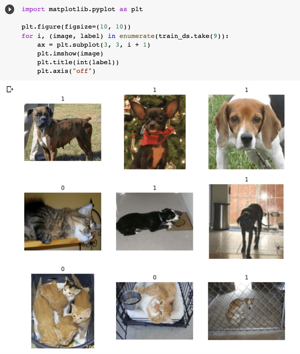
So now let’s look at an example. Since we’ve been speaking so much about cats and dogs, let’s do an Image recognition example on them. 

Load the data

 
So let's first make sure we import the libraries that we need and load the Data.

import numpy as np
import tensorflow as tf
from tensorflow import keras
import tensorflow_datasets as tfds

It is always good to print out your sample size for your training and test to understand how much data you are working with and have a gander with the images, so you can have a look at what data you’re working with. 

Due to images varying in size, it is a good approach to standardise to fixed image size, as it's a good consistent input for the neural network. 

Data pre-processing

 
Now let’s go into Data Augmentation. When working with a smaller dataset, it is good practice to apply random transformation to the training images, such as horizontal flipping. Flipping means rotating an image on a vertical or horizontal axis. This will help expose the model to different angles and aspects of the training data, reducing overfitting. 

from tensorflow import keras
from tensorflow.keras import layers
data_augmentation = keras.Sequential(
   [layers.RandomFlip("horizontal"), layers.RandomRotation(0.1),]
)

Creating a base_model from chosen architecture (Xception)

 
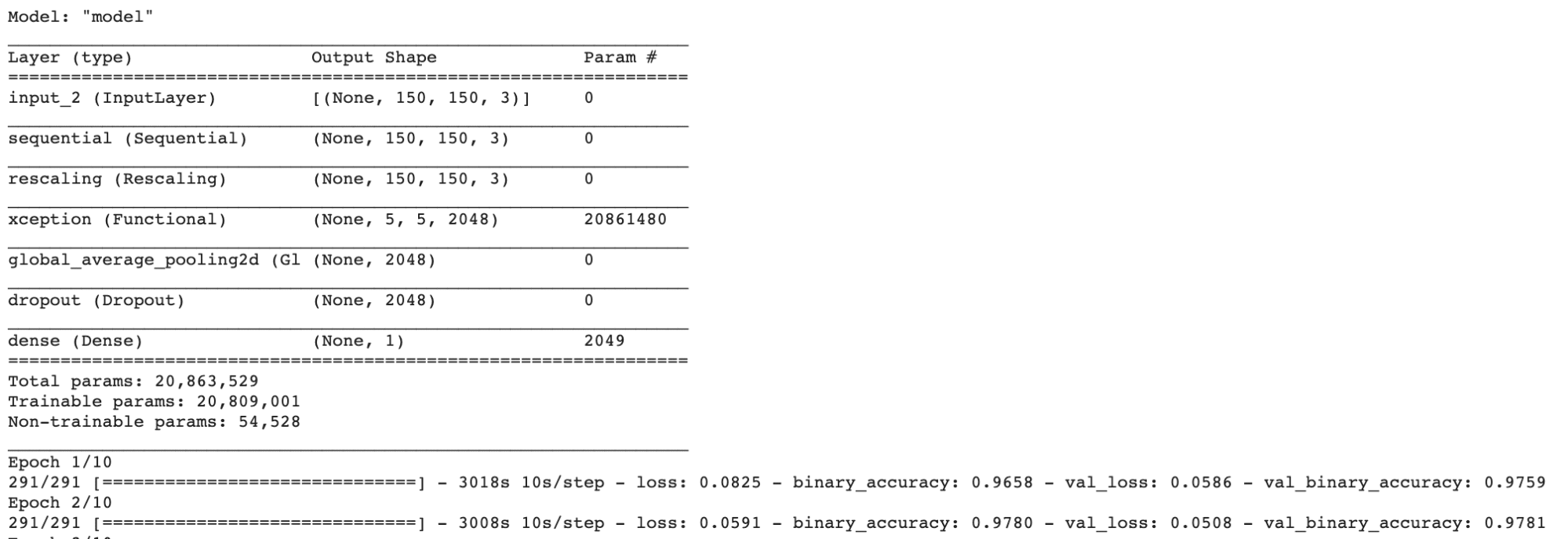
The next step is creating the model. We are first going to start with instantiating a base model, Xception, and loading pre-trained weights into it. In this example, we are using ImageNet. We then move on to freezing all the layers in the base model. Freezing helps to prevent the weights from being updated during training.

base_model = keras.applications.Xception(
   weights="imagenet",  # Weights pre-trained on ImageNet.
   input_shape=(150, 150, 3),
   include_top=False,
)

base_model.trainable = False

Train the top layer

 
The next step is creating a new layer on top of the frozen layers, which will learn its knowledge of the old features and use that to determine predictions on the new dataset. This is beneficial as explained further up in the steps of transfer learning, the likelihood that the current output on the pre-trained model and the output you want from your model will be different is high, therefore adding new layers will improve the model overall. 

# Create a new model on top
inputs = keras.Input(shape=(150, 150, 3))
x = data_augmentation(inputs)  # Apply random data augmentation

Fine-tuning

 
So after we have run the model with frozen layers, we need to run the model with the base models unfrozen, which essentially improves the model, with a lower learning rate. You want to reduce the amount of overfitting, so let’s take this step slowly and unfreeze the base model.

base_model.trainable = True

Now it’s time to compile the model again.

model.compile(
   optimizer=keras.optimizers.Adam(1e-5),  # Low learning rate
   loss=keras.losses.BinaryCrossentropy(from_logits=True),
   metrics=[keras.metrics.BinaryAccuracy()],
)
epochs = 10
model.fit(train_ds, epochs=epochs, validation_data=validation_ds)

If you would like to have a further gander, you can do so by clicking here to view the Colab notebook. 
 
 

Natural Language Processing

 
We’ve spoken quite a bit about image classification, let’s now look into Natural Language Processing (NLP). So what is NLP? NLP is the ability of a computer to be able to detect and understand human language, through speech and text just the way we humans can. 

The human language contains many ambiguities that cause difficulty in being able to create software that can accurately detect speech and text. For example, sarcasm, grammar, and homophones, however, these are just a few bumps in learning the human language. 

Examples of NLP are Speech Recognition and Sentiment Analysis. Use cases of NLP are things like spam detection. I know, you may have never thought of NLP being implemented into spam detection, but it is. NLP’s text classification has the ability to scan emails and detect language that indicates that it could be spam or phishing. It does this by analysing the overuse of bad grammar, threats, overuse of financial terminology, and more. 

So how does Transfer Learning work in NLP? Well, it basically works the same with Image Recognition. Training a natural language model can be quite hefty in price, it requires a lot of data and takes up a lot of training time on fancy hardware. But the good news is that, just like image recognition, you can download these pre-trained models for free along with fine-tuning them to work on your specific dataset.

Where can you find these pre-trained models, you ask?

 
Keras does not only offer pre-trained models for Image recognition, it also provides architectures for NLP. You can have a gander here. 

HuggingFace

 
Let’s look into HuggingFace. HuggingFace is an open-source provider of natural language processing (NLP) which has done an amazing job to make it user-friendly. 

Their Transformers library is a python-based library that provides architectures such as BERT, that perform NLP tasks such as text classification and question answering. All you have to do is load their pre-trained models with just a few lines of code and you are ready to start experimenting. To get started with Transformers, you will need to install it.

Below is an example of using sentiment analysis, which is the ability to be able to identify an opinion expressed in a piece of text.

! pip install transformers

from transformers import pipeline

classifier = pipeline('sentiment-analysis')

classifier('I am finding the article about Transfer learning very useful.')

Output:

[{'label': 'POSITIVE', 'score': 0.9968850016593933}]

Improving your pre-trained model with fine-tuning is an option with HuggingFace, using the Trainer API. Transformers prived a Trainer class which aids in fine-tuning your pre-trained model. This step comes after processing your data and requires you to import TrainingArguments

from transformers import TrainingArguments

To find out more about HuggingFace, you can follow this link. 

Word Embedding

 
How about Word Embedding? What’s that? Word embedding is a representation in which similar words have a similar encoding. It can be able to detect a word in a document and link its relation to other words. 

An example of this is Word2Vec, which is a two-layer neural network that processes texts by vector encoding. 

Word2Vec used two methods to learn word representation:

1. Continuous Bag-of-Words - is a model architecture that tries to predict the target word (middle word) based on the source words (neighbouring words). The order of the words in the context is not necessarily important, the reason the architecture is called ‘bag-of-words
2. Continuous Skip-gram - is a model architecture essentially the opposite of Bag-of-Words. It tries to predict the source words (neighbouring words) given a target word (middle word)

Feature extraction is a strategy used in Word Embedding, where it detects and produces feature representations that are useful for the type of NLP task you are trying to work on. In feature extraction, parts (sentences or words) are extracted to a matrix that has a representation of every word given of every word. The weights do not change and only the top layer of the model is used. 

However, fine-tuning tweaks the pre-trained model’s weights, which can be a detriment as the method can cause a loss in words in the adjustment phase, due to the weights being changed and what was once learned, is no longer in the memory. This is known as ‘catastrophic interference’. 

Example: How to use a pre-trained NLP model in Keras

 
We were just speaking on Word Embedding, so let’s look at an example. To quickly recap what Word Embedding is: it is a representation in which similar words have a similar encoding. It can be able to detect a word in a document and link its relation to other words. So let’s see how this works then.

Load the Data

 
In this example, we are going to look at movie reviews. If you remember the example we did above, using sentiment analysis, produced us an output determining how positive it was. With these movie reviews, we have positive and negative, therefore this is binary classification. 

url = "https://ai.stanford.edu/~amaas/data/sentiment/aclImdb_v1.tar.gz"

dataset = tf.keras.utils.get_file("aclImdb_v1.tar.gz", url,
                                 untar=True, cache_dir='.',
                                 cache_subdir='')

dataset_dir = os.path.join(os.path.dirname(dataset), 'aclImdb')
os.listdir(dataset_dir)

You can see the distinction in the below image, 0 being negative and 1 being positive.

I then moved on to using Embedding Layer from Keras, to turn positive integers into dense vectors with fixed sizes. The weights for the embedding are randomly initialised and are adjusted during backpropagation. Once the knowledge is learnt, the word embeddings will encode similarities between words they have learnt and words they had learnt before.

# Embed a 1,000-word vocabulary into 5 dimensions.

embedding_layer = tf.keras.layers.Embedding(1000, 5)

Text pre-processing

 
During the text pre-processing stage, we are going to initialize a TextVectorization layer with the desired parameters to vectorize movie reviews. The text vectorization layer will help split and map strings from the movie reviews into integers. 

# text vectorization layer to split, and map strings to integers.

vectorize_layer = TextVectorization(
   standardize=custom_standardization,
   max_tokens=vocab_size,
   output_mode='int',
   output_sequence_length=sequence_length)

Create a model

 
The vectorize_layer from the above pre-processing will be implemented as the first layer into the model, as it has transformed the strings into vocabulary indices. It will feed the transformed strings into the Embedding layer. 

The Embedding layer then takes these vocabulary indices and scans through the vector for each word index, where they are learning as the model trains. 

model = Sequential([
 vectorize_layer,
 Embedding(vocab_size, embedding_dim, name="embedding"),
 GlobalAveragePooling1D(),
 Dense(16, activation='relu'),
 Dense(1)
])

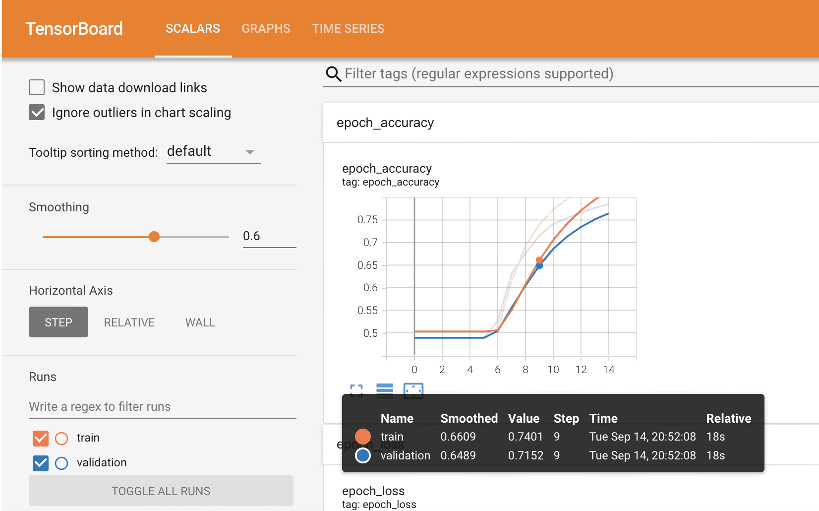
In this example, we are going to use TensorBoard, which is a tool for providing visualisations showing machine learning workflow, for example loss and accuracy. 

Compile the Model

 
We are going to compile the model using the Adam optimizer and BinaryCrossentropy loss.

model.compile(optimizer='adam',
             loss=tf.keras.losses.BinaryCrossentropy(from_logits=True),
             metrics=['accuracy'])

I mentioned the TensorBoard, which visualises the models metrics and you can see this below.

You have seen how to train and test an NLP model using a pre-trained word embedding model. If you would like to have a further look at the Colab notebook, you can do so here. 
 
 

What are the best practices with transfer learning?

1. Pre-trained models - Take advantage of these pre-trained open-source models which can help you solve your target task as they cover different fields. It can save you a lot of time building a model from scratch.
2. Source model - finding a model that is compatible with both your source task and target task is important. If your source model is too far off from your target and little knowledge can get transferred, it will be more time-consuming as the target model will take longer to achieve. 
3. Overfitting - Target tasks with a small data sample, where the source task and target task are too similar, this can lead to overfitting. Freezing layers and tuning the learning rate in the course model can help you reduce overfitting in your model. 

I hope this article has given you a better understanding of how to implement transfer learning through types of Machine Learning. Try it out for yourself!

 
 
Nisha Arya is a Data Scientist and freelance Technical writer. She is particularly interested in providing Data Science career advice or tutorials and theory based knowledge around Data Science. She also wishes to explore the different ways Artificial Intelligence is/can benefit the longevity of human life. A keen learner, seeking to broaden her tech knowledge and writing skills, whilst helping guide others.