 Working With Time Series Using SQL
 Working With Time Series Using SQL
This article is an overview of using SQL to manipulate time series data.
By Michael Grogan, Data Science Consultant
Source: Photo by Tumisu from Pixabay
Tools such as Python or R are most often used to conduct deep time series analysis.
However, knowledge of how to work with time series data using SQL is essential, particularly when working with very large datasets or data that is constantly being updated.
Here are some useful commands that can be invoked in SQL to better work with time series data within the data table itself.
Background
In this example, we are going to work with weather data collected across a range of different times and locations.
The data types in the table of the PostgreSQL database are as below:
weather=# SELECT COLUMN_NAME, DATA_TYPE FROM INFORMATION_SCHEMA.COLUMNS WHERE TABLE_NAME = 'weatherdata';
 column_name |          data_type
-------------+-----------------------------
 date        | timestamp without time zone
 mbhpa       | integer
 temp        | numeric
 humidity    | integer
 place       | character varying
 country     | character varying
 realfeel    | integer
 timezone    | integer
(8 rows)
As you can see, date is defined as a timestamp data type without time zone (which we will also look at in this article).
The variable of interest is temp (temperature) — we are going to look at ways to analyse this variable more intuitively using SQL.
Calculating Moving Averages
Here is a snippet of some of the columns in the data table:
        date         | mbhpa | temp  | humidity
---------------------+-------+-------+----------
 2020-10-12 18:33:24 |  1010 | 13.30 |       74
 2020-10-15 02:12:54 |  1017 |  7.70 |       75
 2020-10-14 23:53:42 |  1016 |  8.80 |       75
 2020-10-15 11:03:25 |  1016 |  9.70 |       75
 2020-10-15 13:05:23 |  1017 | 12.30 |       74
 2020-10-15 18:47:25 |  1015 | 12.10 |       74
 2020-10-16 23:23:23 |  1011 |  9.10 |       75
 2020-10-20 10:25:15 |   967 | 13.80 |       83
 2020-10-27 16:30:30 |   980 | 12.00 |       75
 2020-10-29 15:12:07 |   988 | 11.70 |       75
 2020-10-28 18:42:52 |   990 |  8.80 |       77
Suppose we wish to calculate a moving average of temperature across different time periods.
To do this, we firstly need to make sure that the data is ordered by date, and decide on how many periods should be included in the averaging window.
To start with, a 7-period moving average is used, with all temperature values ordered by date.
>>> select date, avg(temp) OVER (ORDER BY date ROWS BETWEEN 6 PRECEDING AND CURRENT ROW) FROM weatherdata where place='Place Name';        date         |         avg
---------------------+---------------------
 2020-11-12 16:36:40 |  8.8285714285714286
 2020-11-14 15:45:08 |  9.8142857142857143
 2020-11-15 08:53:26 | 10.3857142857142857
 2020-11-17 10:50:32 | 11.2285714285714286
 2020-11-18 14:18:58 | 11.8000000000000000
 2020-11-25 14:54:11 | 11.6285714285714286
 2020-11-25 19:00:21 | 10.9142857142857143
 2020-11-25 19:05:31 | 10.2000000000000000
 2020-11-25 23:41:34 |  9.2857142857142857
 2020-11-26 15:03:10 |  9.4857142857142857
 2020-11-26 17:18:33 |  8.3428571428571429
 2020-11-26 21:30:39 |  7.9142857142857143
 2020-11-26 22:29:17 |  7.6142857142857143
Now, let’s add a 30 and 60-period moving average. We will store these averages along with the 7-period moving average in the one table.
>>> select date, temp, avg(temp) OVER (ORDER BY date ROWS BETWEEN 2 PRECEDING AND CURRENT ROW), avg(temp) OVER (ORDER BY date ROWS BETWEEN 6 PRECEDING AND CURRENT ROW), avg(temp) OVER (ORDER BY date ROWS BETWEEN 29 PRECEDING AND CURRENT ROW), avg(temp) OVER (ORDER BY date ROWS BETWEEN 59 PRECEDING AND CURRENT ROW) FROM weatherdata where place='Place Name';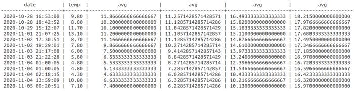
Source: Output Created by Author
More information on how to calculate moving averages within SQL can be found at the following resource by sqltrainingonline.com.
Working with time zones
You will notice that the timestamp contains a date and time. While this is fine when storing just one location in the table, things can get quite tricky when working with locations across multiple time zones.
Note that an integer variable named timezone was created within the table.
Suppose that we are analysing weather patterns across different places with a range of time zones ahead of the inputted time — in this case, all data points were inputted at GMT time.
       date          | timezone
---------------------+----------
 2020-05-09 15:29:00 |       11
 2020-05-09 17:05:00 |       11
 2020-05-09 17:24:00 |       11
 2020-05-10 13:02:00 |       11
 2020-05-13 19:13:00 |       11
 2020-05-10 13:04:00 |       11
 2020-05-10 15:47:00 |       11
 2020-05-13 19:10:00 |       11
 2020-05-14 17:17:00 |       11
 2020-05-09 15:20:00 |        5
 2020-05-09 17:04:00 |        5
 2020-05-09 17:25:00 |        5
 2020-05-09 18:12:00 |        5
 2020-05-10 13:02:00 |        5
 2020-05-10 15:50:00 |        5
 2020-05-10 20:32:00 |        5
 2020-05-11 17:31:00 |        5
 2020-05-13 19:11:00 |        5
 2020-05-17 21:41:00 |       11
 2020-05-15 14:08:00 |       11
 2020-05-14 16:55:00 |        5
 2020-05-15 14:10:00 |        5
(22 rows)
The new times can be calculated as follows:
weather=# select date + interval '1h' * timezone from weatherdata;
      ?column?
---------------------
 2020-05-10 02:29:00
 2020-05-10 04:05:00
 2020-05-10 04:24:00
 2020-05-11 00:02:00
 2020-05-14 06:13:00
 2020-05-11 00:04:00
 2020-05-11 02:47:00
 2020-05-14 06:10:00
 2020-05-15 04:17:00
 2020-05-09 20:20:00
 2020-05-09 22:04:00
 2020-05-09 22:25:00
 2020-05-09 23:12:00
 2020-05-10 18:02:00
 2020-05-10 20:50:00
 2020-05-11 01:32:00
 2020-05-11 22:31:00
 2020-05-14 00:11:00
 2020-05-18 08:41:00
 2020-05-16 01:08:00
 2020-05-14 21:55:00
 2020-05-15 19:10:00
(22 rows)
We can now store the new times as an updated variable, which we will name as newdate.
>>> select date + interval '1h' * (timezone+1) as newdate, temp, mbhpa from weatherdata;      newdate       | temp | mbhpa
--------------------+------+-------
2020-05-10 03:29:00 |  4.2 |  1010
2020-05-10 05:05:00 |  4.1 |  1009
2020-05-10 05:24:00 |  3.8 |  1009
This clause allows us to generate the updated times (which would reflect the actual time in each specific place when variables such as temperature, barometric pressure, etc, were recorded.
Inner Join and Having Clauses
You will notice in the above table that temperature values are included across a range of places.
Suppose that wind speed is also calculated for each place in a separate table.
In this case, we wish to calculate the average temperature across each listed place where the wind speed is higher than 20.
This can be accomplished using the inner join and having clauses as follows:
>>> select t1.place, avg(t1.temp), avg(t2.gust) from weatherdata as t1 inner join wind as t2 on t1.place=t2.place group by t1.place having avg(t2.gust)>'20';      place      |         avg          |         avg
-----------------+----------------------+----------------------
 Place 1         |        17.3          |        22.4
 Place 2         |        14.3          |        26.8
 Place 3         |        7.1           |        27.1
Conclusion
In this article, you have been introduced to some introductory examples of using SQL to work with time series data.
In particular, you saw how to:
- Calculate moving averages
- Work with different time zones
- Calculate averages across different subsets of data
Many thanks for your time and any questions or feedback are greatly appreciated.
Disclaimer: This article is written on an “as is” basis and without warranty. It was written with the intention of providing an overview of data science concepts, and should not be interpreted as professional advice. The findings and interpretations in this article are those of the author and are not endorsed by or affiliated with any third-party mentioned in this article.
Bio: Michael Grogan is a Data Science Consultant. He posesses expertise in time series analysis, statistics, Bayesian modeling, and machine learning with TensorFlow.
Original. Reposted with permission.
Related:
- Multidimensional multi-sensor time-series data analysis framework
- Rejection Sampling with Python
- Deep Learning Is Becoming Overused