Parallelizing Python Code

This article reviews some common options for parallelizing Python code, including process-based parallelism, specialized libraries, ipython parallel, and Ray.

comments

By Dawid Borycki, Biomedical Researcher and Software Engineer & Michael Galarnyk, Data Science Professional

Python is great for tasks like training machine learning models, performing numerical simulations, and quickly developing proof-of-concept solutions without setting up development tools and installing several dependencies. When performing these tasks, you also want to use your underlying hardware as much as possible for quick results. Parallelizing Python code enables this. However, using the standard CPython implementation means you cannot fully use the underlying hardware because of the global interpreter lock (GIL) that prevents running the bytecode from multiple threads simultaneously.

This article reviews some common options for parallelizing Python code including:

For each technique, this article lists some advantages and disadvantages and shows a code sample to help you understand what it’s like to use.

How to Parallelize Python Code

There are several common ways to parallelize Python code. You can launch several application instances or a script to perform jobs in parallel. This approach is great when you don’t need to exchange data between parallel jobs. Otherwise, sharing data between processes significantly reduces performance when aggregating data.

Starting multiple threads within the same process allows you to share data between jobs more efficiently. In this case, thread-based parallelization can offload some work to the background. However, the standard CPython implementation’s global interpreter lock (GIL) prevents running the bytecode in multiple threads simultaneously.

The sample function below simulates complex calculations (meant to mimic activation functions)

iterations_count = round(1e7)
def complex_operation(input_index):
   print("Complex operation. Input index: {:2d}".format(input_index))
   [math.exp(i) * math.sinh(i) for i in [1] * iterations_count]

complex_operation executes several times to better estimate the processing time. It divides the long-running operation into a batch of smaller ones. It does this by dividing the input values into several subsets and then processing the inputs from those subsets in parallel.

Here’s the code that runs complex_operation several times (input range of ten) and measures the execution time with the timebudget package:

@timebudget
def run_complex_operations(operation, input):
   for i in input:
      operation(i) 

input = range(10)
run_complex_operations(complex_operation, input)

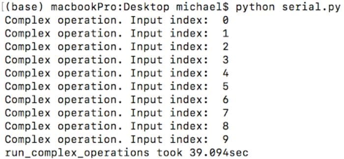
After executing this script, you will get an output similar to the one below:

As you can see, it took about 39 seconds to execute this code on the laptop used in this tutorial. Let’s see how to improve this result.

Process-Based Parallelism

The first approach is to use process-based parallelism. With this approach, it is possible to start several processes at the same time (concurrently). This way, they can concurrently perform calculations.

Starting from Python 3, the multiprocessing package is preinstalled and gives us a convenient syntax for launching concurrent processes. It provides the Pool object, which automatically divides input into subsets and distributes them among many processes.

Here is an example of how to use a Pool object to launch ten processes:

import math
import numpy as np
from timebudget import timebudget
from multiprocessing import Pool

iterations_count = round(1e7)

def complex_operation(input_index):
    print("Complex operation. Input index: {:2d}\n".format(input_index))
    [math.exp(i) * math.sinh(i) for i in [1] * iterations_count]

@timebudget
def run_complex_operations(operation, input, pool):
    pool.map(operation, input)

processes_count = 10

if __name__ == '__main__':
    processes_pool = Pool(processes_count)
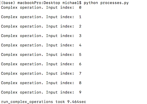
    run_complex_operations(complex_operation, range(10), processes_pool)

Code sample

Each process concurrently performs the complex operation. So, the code could theoretically reduce the total execution time by up to ten times. However, the output from the code below only shows about a fourfold improvement (39 seconds in the previous section vs 9.4 in this section).

There are a couple reasons why the improvement is not tenfold. First, the maximum number of processes that can run concurrently depends on the the number of CPUs in the system. You can find out how many CPUs your system has by using the os.cpu_count() method.

import os
print('Number of CPUs in the system: {}'.format(os.cpu_count()))

The machine used in this tutorial has eight CPUs

The next reason why the improvement is not more is that the computations in this tutorial are relatively small. Finally, it is important to note that there is usually some overhead when parallelizing computation as processes that want to communicate must utilize interprocess communication mechanisms. This means that for very small tasks parallelizing computation is often slower than serial computation (normal Python). If you are interested in learning more about multiprocessing, Selva Prabhakaran has an excellent blog which inspired this section of the tutorial. If you would like to learn about some more of the trade-offs in parallel/distributed computing, check out this tutorial.

Specialized Libraries

Many calculations for specialized libraries like NumPy are unaffected by the GIL and can use threads and other techniques to work in parallel. This section of the tutorial goes over the benefits of combining NumPy and multiprocessing

To demonstrate the differences between the naïve implementation and the NumPy-based implementation, an additional function needs to be implemented:

def complex_operation_numpy(input_index):
      print("Complex operation (numpy). Input index: {:2d}".format(input_index))

      data = np.ones(iterations_count)
      np.exp(data) * np.sinh(data)

The code now uses the NumPy exp and sinh functions to perform calculations on the input sequence. Then, the code executes complex_operation and complex_operation_numpy ten times using the processes pool to compare their performance:

processes_count = 10
input = range(10)

if __name__ == '__main__':
    processes_pool = Pool(processes_count)
    print(‘Without NumPy’)
    run_complex_operations(complex_operation, input, processes_pool)
    print(‘NumPy’)
    run_complex_operations(complex_operation_numpy, input, processes_pool)

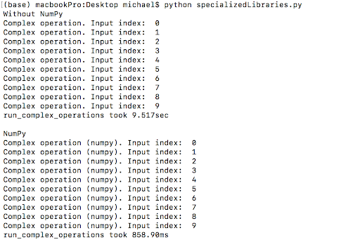
The output below shows the performance with and without NumPy for this script.

NumPy offers a rapid boost in performance. Here, NumPy reduced the computation time to about 10 percent of the original time (859ms vs 9.515sec). One reason why it is faster is because most processing in NumPy is vectorized. With vectorization, the underlying code is effectively “parallelized” because the operation can calculate multiple array elements at once, rather than looping through them one at a time. If you are interested in learning more about this, Jake Vanderplas gave an excellent talk on the subject here.

IPython Parallel

The IPython shell supports interactive parallel and distributed computing across multiple IPython instances. IPython Parallel was developed (almost) together with IPython. When IPython was renamed to Jupyter, they split out IPython Parallel into its own package. IPython Parallel has a number of advantages, but perhaps the biggest advantage is that it enables parallel applications to be developed, executed, and monitored interactively. When using IPython Parallel for parallel computing, you typically start with the ipcluster command.

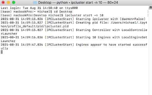
ipcluster start -n 10

The last parameter controls the number of engines (nodes) to launch. The command above becomes available after installing the ipyparallel Python package. Below is a sample output:

The next step is to provide Python code that should connect to ipcluster and start parallel jobs. Fortunately, IPython provides a convenient API for doing this. The code looks like process-based parallelism based on the Pool object:

import math
import numpy as np
from timebudget import timebudget
import ipyparallel as ipp

iterations_count = round(1e7)

def complex_operation(input_index):
    print("Complex operation. Input index: {:2d}".format(input_index))

    [math.exp(i) * math.sinh(i) for i in [1] * iterations_count]

def complex_operation_numpy(input_index):
    print("Complex operation (numpy). Input index: {:2d}".format(input_index))

    data = np.ones(iterations_count)
    np.exp(data) * np.sinh(data)

@timebudget
def run_complex_operations(operation, input, pool):
    pool.map(operation, input)

client_ids = ipp.Client()
pool = client_ids[:]

input = range(10)
print('Without NumPy')
run_complex_operations(complex_operation, input, pool)
print('NumPy')
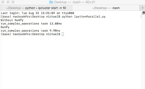
run_complex_operations(complex_operation_numpy, input, pool)

Code sample

The code above executed in a new tab in the terminal produces the output shown below:

The execution times with and without NumPy for IPython Parallel are 13.88 ms and 9.98 ms, respectively. Note, there are no logs included in the standard output, however they can be assessed with additional commands.

Ray

Like IPython Parallel, Ray can be used for parallel and distributed computing. Ray is a fast, simple distributed execution framework that makes it easy to scale your applications and to leverage state of the art machine learning libraries. Using Ray, you can take Python code that runs sequentially and transform it into a distributed application with minimal code changes.

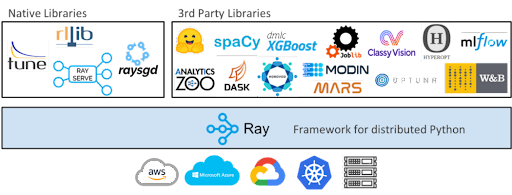
While this tutorial briefly goes over how Ray makes it easy to parallelize plain Python code, it is important to note that Ray and its ecosystem also make it easy to parallelize existing libraries like scikit-learn, XGBoost, LightGBM, PyTorch, and much more.

To use Ray, ray.init() is needed to start all of the relevant Ray processes. By default, Ray creates one worker process per CPU core. If you would want to run Ray on a cluster, you would need to pass in a cluster address with something like ray.init(address='insertAddressHere').

ray.init()

The next step is to create a Ray task. This can be done by decorating a normal Python function with the @ray.remote decorator. This creates a task which can be scheduled across your laptop’s CPU cores (or Ray cluster). Here’s an example for the previously created complex_operation_numpy:

@ray.remote
def complex_operation_numpy(input_index):
   print("Complex operation (numpy). Input index: {:2d}".format(input_index))
   data = np.ones(iterations_count)
   np.exp(data) * np.sinh(data)

In the last step, execute these functions within the ray runtime, like so:

@timebudget
def run_complex_operations(operation, input):
   ray.get([operation.remote(i) for i in input])

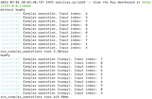
After executing this script, you will get an output similar to the one below:

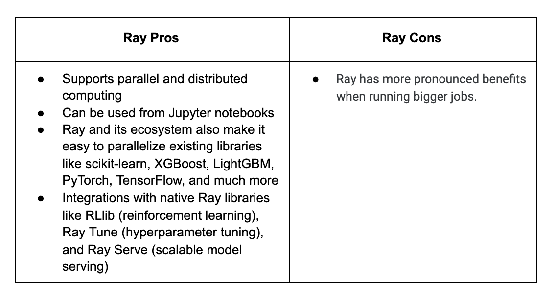
The execution times with and without NumPy for Ray are 3.382sec and 419.98ms, respectively. It is important to remember that the performance benefits of Ray will be more pronounced when executing long-running tasks like the graph below shows.

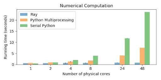
Ray has more pronounced benefits when running bigger jobs (image source)

If you would like to learn about Ray’s syntax, there is an introductory tutorial on it here.

Alternative Python Implementations

One final consideration is that you can apply multithreading using other Python implementations. Examples include IronPython for .NET and Jython for Java. In such cases, you could use the low-level threading support from the underlying frameworks. This approach is beneficial if you already have experience with the multi-processing capabilities of .NET or Java.

Conclusion

This article reviewed common approaches for parallelizing Python through code samples and by highlighting some of their advantages and disadvantages. We performed tests using benchmarks on simple numerical data. It is important to keep in mind that parallelized code often introduces some overhead and that the benefits of parallelization are more pronounced with bigger jobs rather than the short computations in this tutorial.

Keep in mind that the parallelization can be more powerful for other applications. Especially when dealing with typical AI-based tasks in which you must perform repetitive fine-tuning of your models. In such cases, Ray offers the best support due to its rich ecosystem, autoscaling, fault tolerance, and capability of using remote machines.

Dawid Borycki is a Biomedical Researcher and Software Engineer, book author and conference speaker.

Michael Galarnyk is a Data Science Professional, and works in Developer Relations at Anyscale.

Original. Reposted with permission.

Related: