Important Statistics Data Scientists Need to Know

By Lekshmi S. Sunil, IIT Indore '23 | GHC '21 Scholar.

Statistical analysis allows us to derive valuable insights from the data at hand. A sound grasp of the important statistical concepts and techniques is absolutely essential to analyze the data using various tools.

Before we go into the details, let’s take a look at the topics covered in this article:

• Descriptive vs. Inferential Statistics
• Data Types
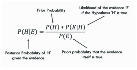
• Probability & Bayes’ Theorem
• Measures of Central Tendency
• Skewness
• Kurtosis
• Measures of Dispersion
• Covariance
• Correlation
• Probability Distributions
• Hypothesis Testing
• Regression

 

Descriptive vs. Inferential Statistics

 

Statistics as a whole deals with the collection, organization, analysis, interpretation, and presentation of data. Within statistics, there are two main branches:

1. Descriptive Statistics: This involves describing the features of the data, organizing and presenting the data either visually through charts/graphs or through numerical calculations using measures of central tendency, variability, and distribution. One noteworthy point is that conclusions are drawn based on already known data.
2. Inferential Statistics: This involves drawing inferences and making generalizations about larger populations using samples taken from them. Hence, more complex calculations are required. The final results are produced using techniques like hypothesis testing, correlation, and regression analysis. Predicted future outcomes and conclusions drawn go beyond the level of available data.

 

Data Types

 

To perform proper Exploratory Data Analysis(EDA) applying the most appropriate statistical techniques, we need to understand what type of data we are working on.

1. Categorical Data

Categorical data represents qualitative variables like an individual’s gender, blood group, mother tongue etc. Categorical data also be in the form of numerical values without any mathematical meaning. For example, if gender is the variable, a female can be represented by 1 and male by 0.

• Nominal data: Values label the variables, and there is no defined hierarchy between the categories, i.e., there is no order or direction—for example, religion, gender etc. Nominal scales with only two categories are termed “dichotomous”.
• Ordinal data: Order or hierarchy exists between the categories—for example, quality ratings, education level, student letter grades etc.

2. Numerical Data

Numerical data represents quantitative variables expressed only in terms of numbers. For example, an individual’s height, weight etc.

• Discrete data: Values are countable and are integers (most often whole numbers). For example, the number of cars in a parking lot, no of countries etc.
• Continuous data: Observations can be measured but can’t be counted. Data assumes any value within a range—for example, weight, height etc. Continuous data can be further divided into interval data(ordered values having the same differences between them but has no true zero) and ratio data (ordered values having the same differences between them and true zero exists).

 

Probability & Bayes’ Theorem

 

Probability is the measure of the likelihood that an event will occur.

• P(A) + P(A’) = 1
• P(A∪B) = P(A) + P(B) − P(A∩B)
• Independent Events: Two events are independent if the occurrence of one does not affect the probability of occurrence of the other. P(A∩B) = P(A)P(B) where P(A) != 0 and P(B) != 0.
• Mutually Exclusive Events: Two events are mutually exclusive or disjoint if they cannot both occur at the same time. P(A∩B) = 0 and P(A∪B) = P(A)+P(B).
• Conditional Probability: Probability of an event A, given that another event B has already occurred. This is represented by P(A|B). P(A|B) = P(A∩B)/P(B), when P(B)>0.
• Bayes’ Theorem

 

Measures of Central Tendency

 

Import the statistics module.

• Mean: Average value of the dataset.

numpy.mean( ) can also be used.

• Median: Middle value of the dataset.

numpy.median( ) can also be used.

• Mode: Most frequent value in the dataset.

When to use mean, median, and mode?

Relation between mean, median, and mode: Mode = 3 Median — 2 Mean

 

Skewness

 

A measure of symmetry, or more precisely, lack of symmetry (asymmetry).

• Normal/symmetric distribution: mode = median = mean
• Positively (right) skewed distribution: mode < median < mean
• Negatively (left) skewed distribution: mean < median < mode

 

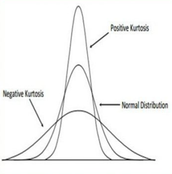
Kurtosis

 

A measure of whether the data is heavy-tailed or light-tailed relative to a normal distribution, i.e., it measures the “tailedness” or “peakedness” of a distribution.

• Leptokurtic - positive kurtosis
• Mesokurtic - normal distribution
• Platykurtic - negative kurtosis

Skewness and kurtosis using Python.

 

Measures of Dispersion

 

Describes the spread/scattering of data around a central value.

Range: The difference between the largest and the smallest value in the dataset.

Quartile Deviation: The quartiles of a data set divide the data into four equal parts—the first quartile (Q1) is the middle number between the smallest number and the median of the data. The second quartile (Q2) is the median of the data set. The third quartile (Q3) is the middle number between the median and the largest number. Quartile deviation is Q = ½ × (Q3 — Q1)

Interquartile Range: IQR = Q3 — Q1

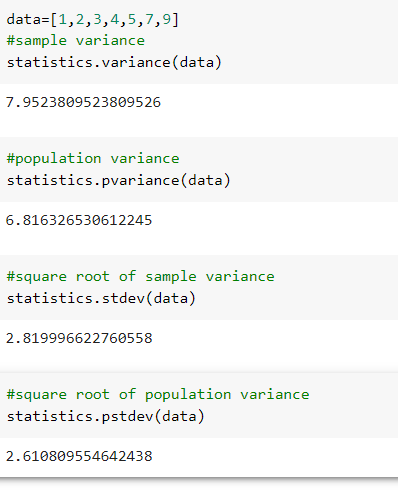
Variance: The average squared difference between each data point and the mean. Measures how spread out the dataset is relative to the mean.

Standard deviation: Square root of variance.

Variance and standard deviation using Python.

 

Covariance

 

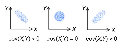
It is the relationship between a pair of random variables where a change in one variable causes change in another variable.

Negative, zero, and positive covariance.

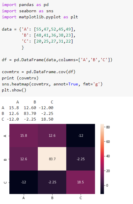
Covariance matrix and its heatmap representation using Python.

 

Correlation

 

It shows whether and how strongly a pair of variables are related to each other.

Correlation matrix using the same data used for covariance.

Covariance vs. Correlation.

 

Probability Distributions

 

There are two broad types of probability distributions — Discrete & Continuous probability distributions.

Discrete Probability Distribution:

• Bernoulli Distribution

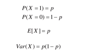
A random variable takes a single trial with only two possible outcomes: 1 (success) with probability p and 0 (failure) with probability 1-p.

• Binomial Distribution

Each trial is independent. There are only two possible outcomes in a trial- either a success or a failure. A total number of n identical trials are conducted. The probability of success and failure is the same for all trials. (Trials are identical.)

• Poisson Distribution

Measures the probability of a given number of events happening in a specified time period.

Continuous Probability Distribution:

• Uniform Distribution

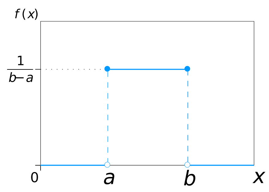
Also called rectangular distribution. All outcomes are equally likely.

• Normal/Gaussian Distribution

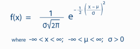
The mean, median, and mode of the distribution coincide. The curve of the distribution is bell-shaped and symmetrical about the line x = μ. The total area under the curve is 1. Exactly half of the values are to the left of the center and the other half to the right.

A normal distribution is highly different from Binomial Distribution. However, if the number of trials approaches infinity, then the shapes will be quite similar.

• Exponential Distribution

Probability distribution of the time between events in a Poisson point process, i.e., a process in which events occur continuously and independently at a constant average rate.

 

Hypothesis Testing

 

First, let’s take a look at the difference between the null hypothesis and the alternative hypothesis.

Null hypothesis: Statement about the population parameter that is either believed to be true or is used to put forth an argument unless it can be shown to be incorrect by hypothesis testing.

Alternative hypothesis: Claim about the population that is contradictory to the null hypothesis and what we conclude if we reject the null hypothesis.

Type I error: Rejection of a true null hypothesis

Type II error: Non-rejection of a false null hypothesis

Significance level (α): Probability of rejecting the null hypothesis when it is true.

p-value: Probability of the test statistic being at least as extreme as the one observed given that the null hypothesis is true.

• When p-value > α, we fail to reject the null hypothesis.
• While p-value ≤ α, we reject the null hypothesis, and we can conclude that we have a significant result.

In statistical hypothesis testing, a result has statistical significance when it is very unlikely to have occurred given the null hypothesis.

Critical value: A point on the scale of the test statistic beyond which we reject the null hypothesis. It depends upon a test statistic, which is specific to the type of test, and the significance level, α, which defines the sensitivity of the test.

 

Linear Regression

 

Linear Regression is usually the first ML algorithm that we come across. It is simple, and understanding it lays the foundation for other advanced ML algorithms.

Simple Linear Regression

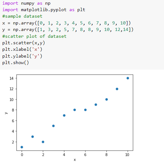
Linear approach to modeling the relationship between a dependent variable and one independent variable.

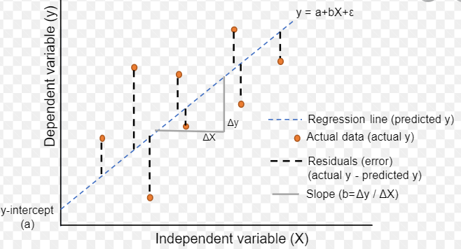
We have to find the parameters so that the model best fits the data. The regression line (i.e., the best fit line) is the line for which the error between the predicted values and the observed values is minimum.

Regression line.

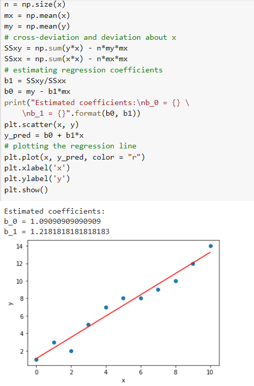
Now, let’s try to implement this.

Multiple Linear Regression

Linear approach to modeling the relationship between a dependent variable and two or more independent variables.

Original. Reposted with permission.

 

Related:

• 11 Important Probability Distributions Explained
• Hypothesis Testing Explained
• Top 3 Statistical Paradoxes in Data Science