A Gentle Introduction to Support Vector Machines
A guide to understanding support vector machines for classification: from theory to scikit-learn implementation.
Image by Author
Support vector machines, commonly called SVM, are a class of simple yet powerful machine learning algorithms used in both classification and regression tasks. In this discussion, we’ll focus on the use of support vector machines for classification.
We’ll start by looking at the basics of classification and hyperplanes that separate classes. We’ll then go over maximum margin classifiers, gradually building up to support vector machines and the scikit-learn implementation of the algorithm.
Classification Problem and Separating Hyperplanes
Classification is a supervised learning problem where we have labeled data points and the goal of the machine learning algorithm is to predict the label of a new data point.
For simplicity, let's take a binary classification problem with two classes, namely, class A and class B. And we need to find a hyperplane that separates these two classes.
Mathematically, a hyperplane is a subspace whose dimension is one less than the ambient space. Meaning if the ambient space is a line, the hyperplane is a point. And if the ambient space is a two-dimensional plane, the hyperplane is a line, and so on.
So when we have a hyperplane separating the two classes, the data points belonging to class A lie on one side of the hyperplane. And those belonging to class B lie on the other side.
Therefore, in one-dimensional space, the separating hyperplane is a point:
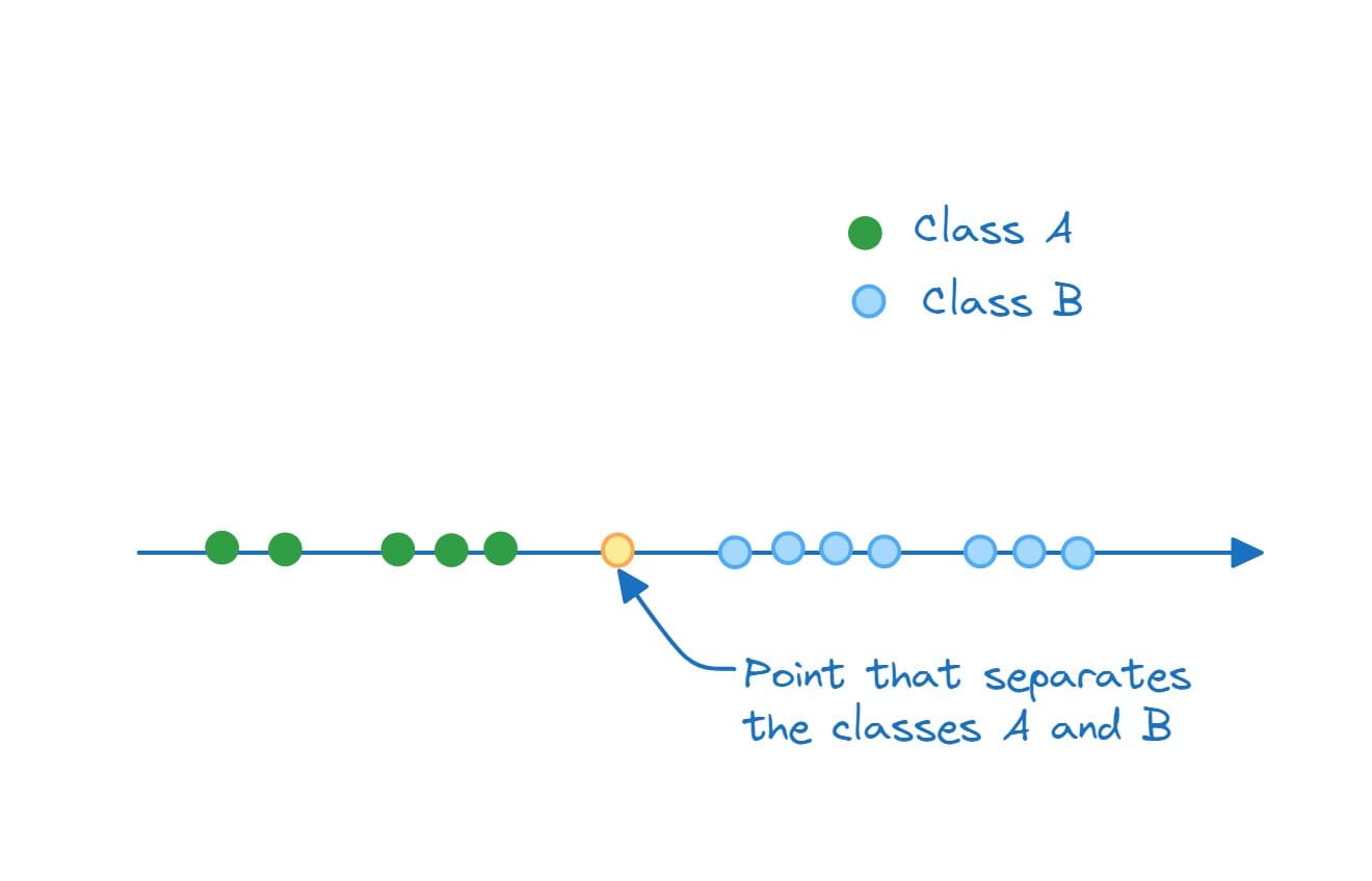
Separating Hyperplane in 1D (A Point) | Image by Author
In two dimensions, the hyperplane that separates class A and class B is a line:
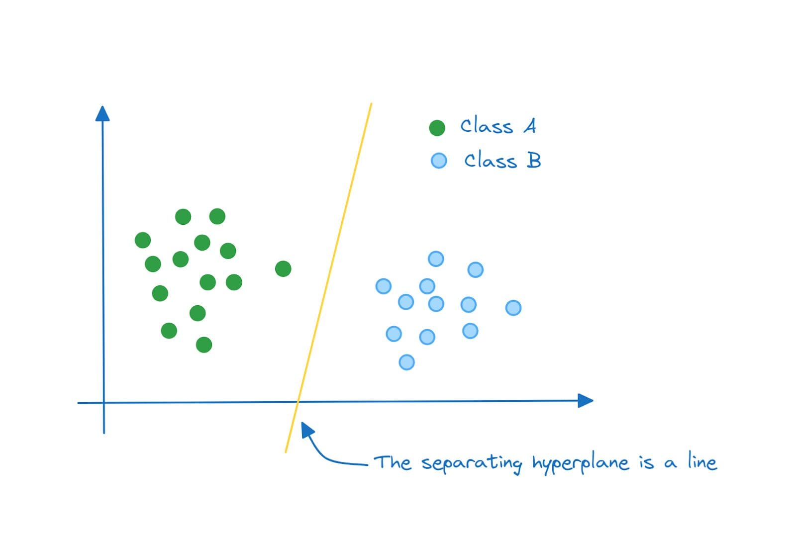
Separating Hyperplane in 2D (A Line) | Image by Author
And in three dimensions, the separating hyperplane is a plane:
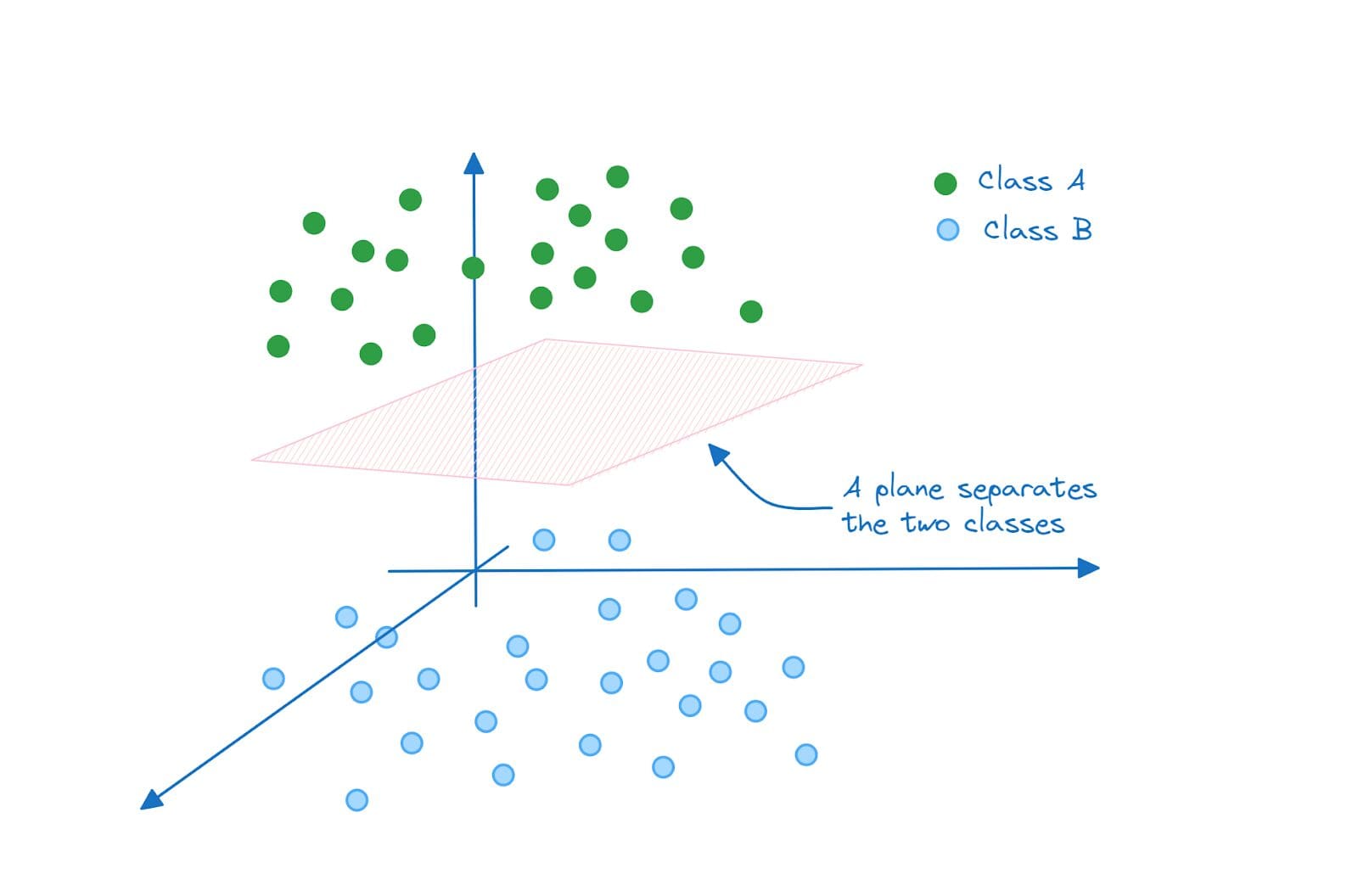
Separating Hyperplane in 3D (A Plane) | Image by Author
Similarly in N dimensions the separating hyperplane will be an (N-1)-dimensional subspace.
If you take a closer look, for the two dimensional space example, each of the following is a valid hyperplane that separates the classes A and B:
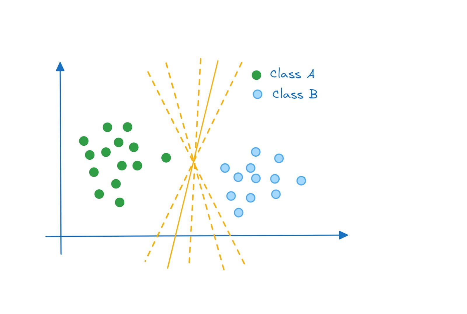
Separating Hyperplanes | Image by Author
So how do we decide which hyperplane is the most optimal? Enter maximum margin classifier.
Maximum Margin Classifier
The optimal hyperplane is the one that separates the two classes while maximizing the margin between them. And a classifier that functions thus is called a maximum margin classifier.
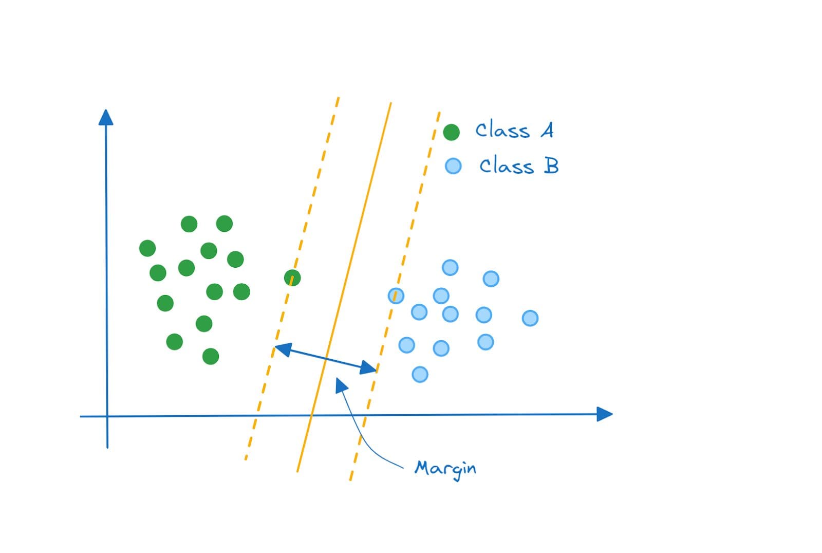
Maximum Margin Classifier | Image by Author
Hard and Soft Margins
We considered a super simplified example where the classes were perfectly separable and the maximum margin classifier was a good choice.
But what if your data points were distributed like this? The classes are still perfectly separable by a hyperplane, and the hyperplane that maximizes the margin will look like this:

Is the Maximum Margin Classifier Optimal? | Image by Author
But do you see the problem with this approach? Well, it still achieves class separation. However, this is a high variance model that is, perhaps, trying to fit the class A points too well.
Notice, however, that the margin does not have any misclassified data point. Such a classifier is called a hard margin classifier.
Take a look at this classifier instead. Won't such a classifier perform better? This is a substantially lower variance model that would do reasonably well on classifying both points from class A and class B.
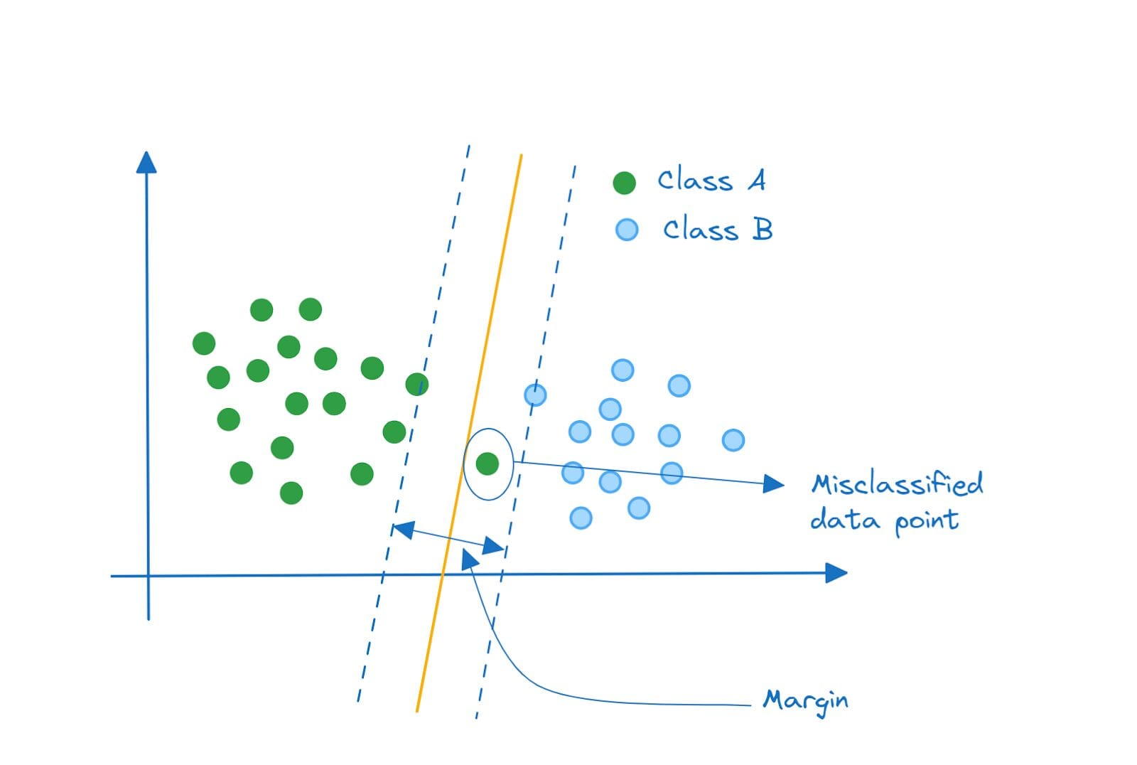
Linear Support Vector Classifier | Image by Author
Notice that we have a misclassified data point inside the margin. Such a classifier that allows minimal misclassifications is a soft margin classifier.
Support Vector Classifier
The soft margin classifier we have is a linear support vector classifier. The points are separable by a line (or a linear equation). If you’ve been following along so far, it should be clear what support vectors are and why they are called so.
Each data point is a vector in the feature space. The data points that are closest to the separating hyperplane are called support vectors because they support or aid the classification.
It's also interesting to note that if you remove a single data point or a subset of data points that are not support vectors, the separating hyperplane does not change. But, if you remove one or more support vectors, the hyperplane changes.
In the examples so far, the data points were linearly separable. So we could fit a soft margin classifier with the least possible error. But what if the data points were distributed like this?
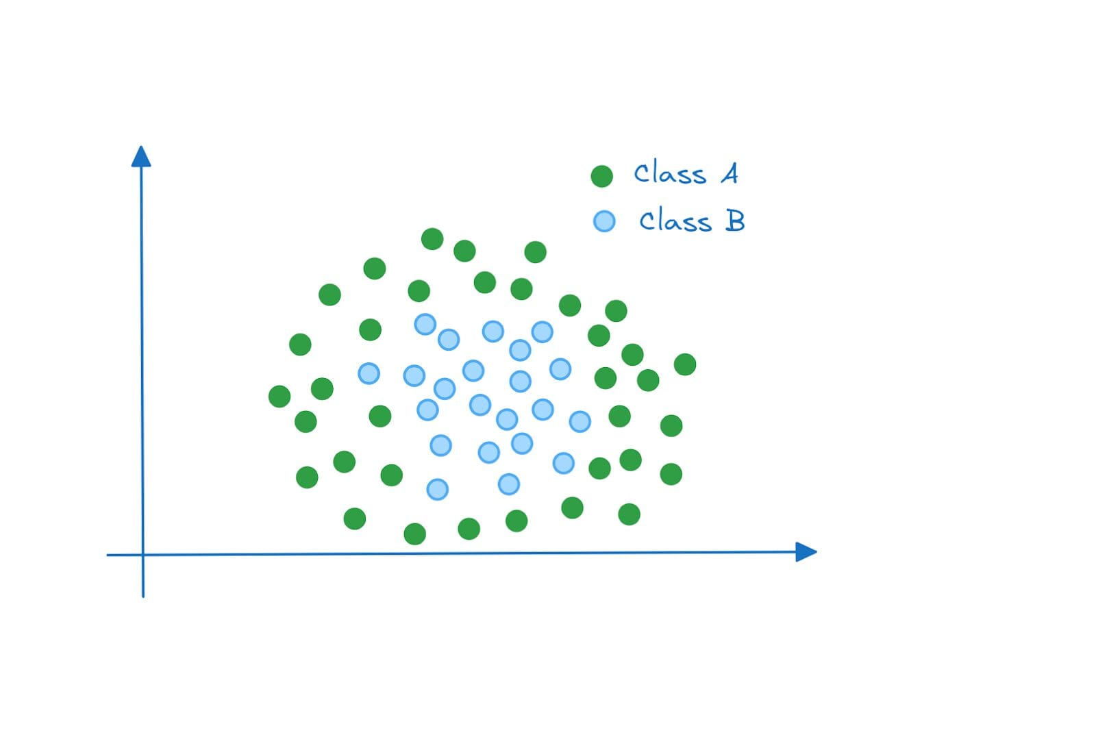
Non-linearly Separable Data | Image by Author
In this example, the data points are not linearly separable. Even if we have a soft margin classifier that allows for misclassification, we will not be able to find a line (separating hyperplane) that achieves good performance on these two classes.
So what do we do now?
Support Vector Machines and the Kernel Trick
Here’s a summary of what we’d do:
- Problem: The data points are not linearly separable in the original feature space.
- Solution: Project the points onto a higher dimensional space where they are linearly separable.
But projecting the points onto a higher dimensional features space requires us to map the data points from the original feature space to the higher dimensional space.
This recomputation comes with non-negligible overhead, especially when the space that we want to project onto is of much higher dimensions than the original feature space. Here's where the kernel trick comes into play.
Mathematically, the support vector classifier you can be represented by the following equation [1]:
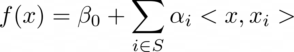
Here,  is a constant, and indicates that we sum over the set of indices corresponding to the support points.
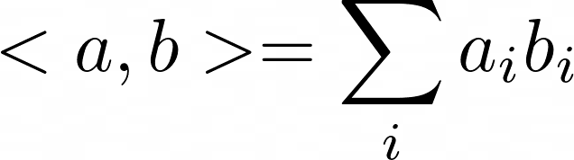
is the inner product between the points and . The inner product between any two vectors a and b is given by:
The kernel function K(.) allows to generalize the linear support vector classifier to non-linear cases. We replace the inner product with the kernel function:
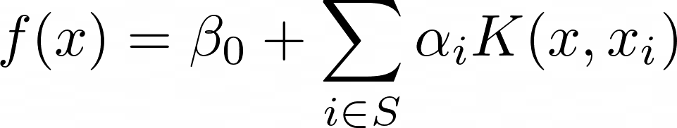
The kernel function accounts for the non-linearity. And also allows for computations to be performed—on the data points in the original features space—without having to recompute them in the higher dimensional space.
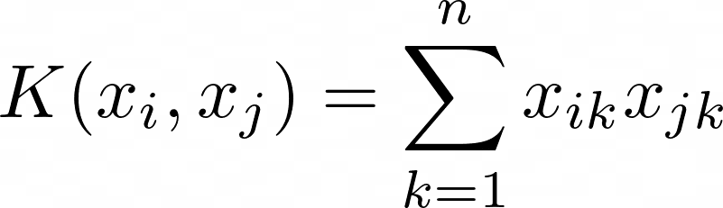
For the linear support vector classifier, the kernel function is simply the inner product and takes the following form:
Support Vector Machines in Scikit-Learn
Now that we understand the intuition behind support vector machines, let's code a quick example using the scikit-learn library.
The svm module in the scikit-learn library comes with implementations of classes like Linear SVC, SVC, and NuSVC. These classes can be used for both binary and multiclass classification. Scikit-learn’s extended docs lists the supported kernels.
We’ll use the built-in wine dataset. It’s a classification problem where the features of wine are used to predict the output label which is one of the three classes: 0, 1, or 2. It’s a small dataset with about 178 records and 13 features.
Here, we’ll only focus on:
- loading and preprocessing the data and
- fitting the classifier to the dataset
Step 1 – Import the Necessary Libraries and Load the Dataset
First, let’s load the wine dataset available in scikit-learn’s datasets module:
from sklearn.datasets import load_wine

# Load the wine dataset
wine = load_wine()
X = wine.data
y = wine.target
Step 2 – Split the Dataset Into Training and Test Datasets
Let’s split the dataset into train and test sets. Here, we use an 80:20 split where 80% and 20% of the data points go into the train and test datasets, respectively:
from sklearn.model_selection import train_test_split

# Split the dataset into training and test sets
X_train, X_test, y_train, y_test = train_test_split(X, y, test_size=0.2, random_state=10)
Step 3 – Preprocess the Dataset
Next, we preprocess the dataset. We use a StandardScaler to transform the data points such that they follow a distribution with zero mean and unit variance:
# Data preprocessing
from sklearn.preprocessing import StandardScaler

scaler = StandardScaler()
X_train_scaled = scaler.fit_transform(X_train)
X_test_scaled = scaler.transform(X_test)
Remember not to use fit_transform on the test dataset as it would lead to the subtle problem of data leakage.
Step 4 – Instantiate an SVM Classifier and Fit it to the Training Data
We’ll use SVC for this example. We instantiate svm, an SVC object, and fit it to the training data:
from sklearn.svm import SVC

# Create an SVM classifier
svm = SVC()

# Fit the SVM classifier to the training data
svm.fit(X_train_scaled, y_train)
Step 5 – Predict the Labels for the Test Samples
To predict the class labels for the test data, we can call the predict method on the svm object:
# Predict the labels for the test set
y_pred = svm.predict(X_test_scaled)
Step 6 – Evaluate the Accuracy of the Model
To wrap up the discussion, we’ll only compute the accuracy score. But we can also get a much detailed classification report and confusion matrix.
from sklearn.metrics import accuracy_score

# Calculate the accuracy of the model
accuracy = accuracy_score(y_test, y_pred)
print(f"{accuracy=:.2f}")
Output >>> accuracy=0.97
Here’s the complete code:
from sklearn.datasets import load_wine
from sklearn.model_selection import train_test_split
from sklearn.preprocessing import StandardScaler
from sklearn.svm import SVC
from sklearn.metrics import accuracy_score

# Load the wine dataset
wine = load_wine()
X = wine.data
y = wine.target

# Split the dataset into training and test sets
X_train, X_test, y_train, y_test = train_test_split(X, y, test_size=0.2, random_state=10)

# Data preprocessing
from sklearn.preprocessing import StandardScaler

scaler = StandardScaler()
X_train_scaled = scaler.fit_transform(X_train)
X_test_scaled = scaler.transform(X_test)

# Create an SVM classifier
svm = SVC()

# Fit the SVM classifier to the training data
svm.fit(X_train_scaled, y_train)

# Predict the labels for the test set
y_pred = svm.predict(X_test_scaled)

# Calculate the accuracy of the model
accuracy = accuracy_score(y_test, y_pred)
print(f"{accuracy=:.2f}")
We have a simple support vector classifier. There are hyperparameters that you can tune to improve the performance of the support vector classifier. Commonly tuned hyperparameters include the regularization constant C and the gamma value.
Conclusion
I hope you found this introductory guide to support vector machines helpful. We covered just enough intuition and concepts to understand how support vector machines work. If you’re interested in diving deeper, you can check the references linked to below. Keep learning!
References and Learning Resources
[1] Chapter on Support Vector Machines, An Introduction to Statistical Learning (ISLR)
[2] Chapter on Kernel Machines, Introduction to Machine Learning
[3] Support Vector Machines, scikit-learn docs
Bala Priya C is a developer and technical writer from India. She likes working at the intersection of math, programming, data science, and content creation. Her areas of interest and expertise include DevOps, data science, and natural language processing. She enjoys reading, writing, coding, and coffee! Currently, she's working on learning and sharing her knowledge with the developer community by authoring tutorials, how-to guides, opinion pieces, and more.