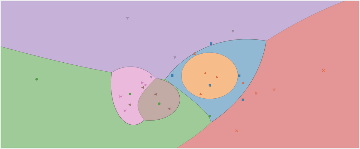
The decision region of a Gaussian naive Bayes classifier. Image by the Author.

I think this is a classic at the beginning of each data science career: the Naive Bayes Classifier. Or I should rather say the family of naive Bayes classifiers, as they come in many flavors. For example, there is a multinomial naive Bayes, a Bernoulli naive Bayes, and also a Gaussian naive Bayes classifier, each different in only one small detail, as we will find out. The naive Bayes algorithms are quite simple in design but proved useful in many complex real-world situations.

In this article, you can learn

• how the naive Bayes classifiers work,
• why it makes sense to define them the way they are and
• how to implement them in Python using NumPy.

You can find the code on my Github.

It might help a bit to check out my primer on Bayesian statistics A gentle Introduction to Bayesian Inference to get used to the Bayes formula. As we will implement the classifier in a scikit learn-conform way, it’s also worthwhile to check out my article Build your own custom scikit-learn Regression. However, the scikit-learn overhead is quite small and you should be able to follow along anyway.

We will start exploring the astonishingly simple theory of naive Bayes classification and then turn to the implementation.

The Theory

What are we really interested in when classifying? What are we actually doing, what is the input and the output? The answer is simple:

Given a data point x, what is the probability of x belonging to some class c?

That’s all we want to answer with any classification. You can directly model this statement as a conditional probability: p(c|x).

For example, if there are

• 3 classes c₁, c₂, c₃, and
• x consists of 2 features x₁, x₂,

the result of a classifier could be something like p(c₁|x₁, x₂)=0.3, p(c₂|x₁, x₂)=0.5 and p(c₃|x₁, x₂)=0.2. If we care for a single label as the output, we would choose the one with the highest probability, i.e. c₂ with a probability of 50% here.

The naive Bayes classifier tries to compute these probabilities directly.

Naive Bayes

Ok, so given a data point x, we want to compute p(c|x) for all classes c and then output the c with the highest probability. In formulas you often see this as

Image by the Author.

Note: max p(c|x) returns the maximum probability while argmax p(c|x) returns the c with this highest probability.

But before we can optimize p(c|x), we have to be able to compute it. For this, we use Bayes’ theorem:

Bayes theorem. Image by the Author.

This is the Bayes part of naive Bayes. But now, we have the following problem: What are p(x|c) and p(c)?

This is what the training of a naive Bayes classifier is all about.

The Training

To illustrate everything, let us use a toy dataset with two real features x₁, x₂, and three classes c₁, c₂, c₃ in the following.

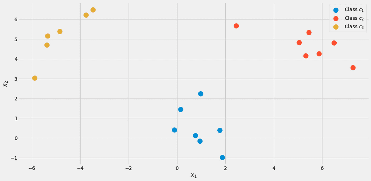
The data, visualized. Image by the Author.

You can create this exact dataset via

from sklearn.datasets import make_blobs

X, y = make_blobs(n_samples=20, centers=[(0,0), (5,5), (-5, 5)], random_state=0)

Let us start with the class probability p(c), the probability that some class c is observed in the labeled dataset. The simplest way to estimate this is to just compute the relative frequencies of the classes and use them as the probabilities. We can use our dataset to see what this means exactly.

There are 7 out of 20 points labeled class c₁ (blue) in the dataset, therefore we say p(c₁)=7/20. We have 7 points for class c₂ (red) as well, therefore we set p(c₂)=7/20. The last class c₃ (yellow) has only 6 points, hence p(c₃)=6/20.

This simple calculation of the class probabilities resembles a maximum likelihood approach. You can, however, also use another prior distribution, if you like. For example, if you know that this dataset is not representative of the true population because class c₃ should appear in 50% of the cases, then you set p(c₁)=0.25, p(c₂)=0.25 and p(c₃)=0.5. Whatever helps you improving the performance on the test set.

We now turn to the likelihood p(x|c)=p(x₁, x₂|c). One approach to calculate this likelihood is to filter the dataset for samples with label c and then try to find a distribution (e.g. a 2-dimensional Gaussian) that captures the features x₁, x₂.

Unfortunately, usually, we don’t have enough samples per class to do a proper estimation of the likelihood.

To be able to build a more robust model, we make the naive assumption that the features x₁, x₂ are stochastically independent, given c. This is just a fancy way of making the math easier via

Image by the Author

for every class c. This is where the naive part of naive Bayes comes from because this equation does not hold in general. Still, even then the naive Bayes yields good, sometimes outstanding results in practice. Especially for NLP problems with bag-of-words features, the multinomial naive Bayes shines.

The arguments given above are the same for any naive Bayes classifier you can find. Now it just depends on how you model p(x₁|c₁), p(x₂|c₁), p(x₁|c₂), p(x₂|c₂), p(x₁|c₃) and p(x₂|c₃).

If your features are 0 and 1 only, you could use a Bernoulli distribution. If they are integers, a Multinomial distribution. However, we have real feature values and decide for a Gaussian distribution, hence the name Gaussian naive Bayes. We assume the following form

Image by the Author.

where μᵢ,ⱼ is the mean and σᵢ,ⱼ is the standard deviation that we have to estimate from the data. This means that we get one mean for each feature i coupled with a class cⱼ, in our case 2*3=6 means. The same goes for the standard deviations. This calls for an example.

Let us try to estimate μ₂,₁ and σ₂,₁. Because j=1, we are only interested in class c₁, let us only keep samples with this label. The following samples remain:

# samples with label = c_1

array([[ 0.14404357,  1.45427351],

[ 0.97873798,  2.2408932 ],

[ 1.86755799, -0.97727788],

[ 1.76405235,  0.40015721],

[ 0.76103773,  0.12167502],

[-0.10321885,  0.4105985 ],

[ 0.95008842, -0.15135721]])

Now, because of i=2 we only have to consider the second column. μ₂,₁ is the mean and σ₂,₁ the standard deviation for this column, i.e. μ₂,₁ = 0.49985176 and σ₂,₁ = 0.9789976.

These numbers make sense if you look at the scatter plot from above again. The features x₂ of the samples from class c₁ are around 0.5, as you can see from the picture.

We compute this now for the other five combinations and we are done!

In Python, you can do it like this:

from sklearn.datasets import make_blobs
import numpy as np

# Create the data. The classes are c_1=0, c_2=1 and c_3=2.
X, y = make_blobs(
    n_samples=20, centers=[(0, 0), (5, 5), (-5, 5)], random_state=0
)

# The class probabilities.
# np.bincounts counts the occurence of each label.
prior = np.bincount(y) / len(y)

# np.where(y==i) returns all indices where the y==i.
# This is the filtering step.
means = np.array([X[np.where(y == i)].mean(axis=0) for i in range(3)])
stds = np.array([X[np.where(y == i)].std(axis=0) for i in range(3)])

We receive

# priors
array([0.35, 0.35, 0.3 ])
# means 
array([[ 0.90889988,  0.49985176],
       [ 5.4111385 ,  4.6491892 ],
       [-4.7841679 ,  5.15385848]])
# stds
array([[0.6853714 , 0.9789976 ],
       [1.40218915, 0.67078568],
       [0.88192625, 1.12879666]])

This is the result of the training of a Gaussian naive Bayes classifier.

Making Predictions

The complete prediction formula is

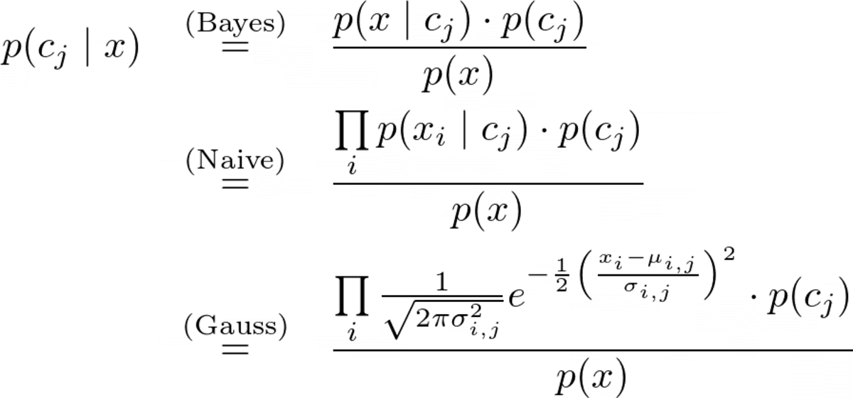
Image by the Author.

Let’s assume a new data point x*=(-2, 5) comes in.

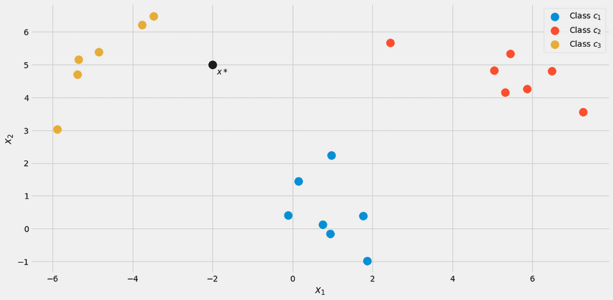
Image by the Author.

To see which class it belongs to, let us compute p(c|x*) for all classes. From the picture, it should belong to class c₃ = 2, but let’s see. Let us ignore the denominator p(x) for a second. Using the following loop computed the nominators for j = 1, 2, 3.

x_new = np.array([-2, 5])

for j in range(3):
    print(
        f"Probability for class {j}: {(1/np.sqrt(2*np.pi*stds[j]**2)*np.exp(-0.5*((x_new-means[j])/stds[j])**2)).prod()*p[j]:.12f}"
    )

We receive

Probability for class 0: 0.000000000263
Probability for class 1: 0.000000044359
Probability for class 2: 0.000325643718

Of course, these probabilities (we shouldn’t call them that way) don’t add up to one since we ignored the denominator. However, this is no problem since we can just take these unnormalized probabilities and divide them by their sum, then they will add up to one. So, dividing these three values by their sum of about 0.00032569, we get

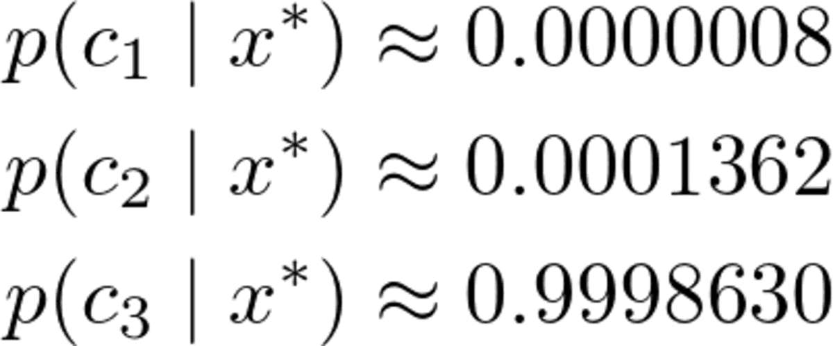
Image by the Author.

A clear winner, as we expected. Now, let us implement it!

The Complete Implementation

This implementation is by far not efficient, not numerically stable, it only serves an educational purpose. We have discussed most of the things, so it should be easy to follow along now. You can ignore all the check functions, or read my article Build your own custom scikit-learn if you are interested in what they exactly do.

Just note that I implemented a predict_proba method first to compute probabilities. The method predict just calls this method and returns the index (=class) with the highest probability using an argmax function (there it is again!). The class awaits classes from 0 to k-1, where k is the number of classes.

import numpy as np
from sklearn.base import BaseEstimator, ClassifierMixin
from sklearn.utils.validation import check_X_y, check_array, check_is_fitted


class GaussianNaiveBayesClassifier(BaseEstimator, ClassifierMixin):
    def fit(self, X, y):
        X, y = check_X_y(X, y)
        self.priors_ = np.bincount(y) / len(y)
        self.n_classes_ = np.max(y) + 1

        self.means_ = np.array(
            [X[np.where(y == i)].mean(axis=0) for i in range(self.n_classes_)]
        )
        self.stds_ = np.array(
            [X[np.where(y == i)].std(axis=0) for i in range(self.n_classes_)]
        )

        return self

    def predict_proba(self, X):
        check_is_fitted(self)
        X = check_array(X)

        res = []
        for i in range(len(X)):
            probas = []
            for j in range(self.n_classes_):
                probas.append(
                    (
                        1
                        / np.sqrt(2 * np.pi * self.stds_[j] ** 2)
                        * np.exp(-0.5 * ((X[i] - self.means_[j]) / self.stds_[j]) ** 2)
                    ).prod()
                    * self.priors_[j]
                )
            probas = np.array(probas)
            res.append(probas / probas.sum())
        return np.array(res)

    def predict(self, X):
        check_is_fitted(self)
        X = check_array(X)

        res = self.predict_proba(X)

        return res.argmax(axis=1)

Testing the Implementation

While the code is quite short it is still too long to be completely sure that we didn’t do any mistakes. So, let us check how it fares against the scikit-learn GaussianNB classifier.

my_gauss = GaussianNaiveBayesClassifier()
my_gauss.fit(X, y)
my_gauss.predict_proba([[-2, 5], [0,0], [6, -0.3]])

outputs

array([[8.06313823e-07, 1.36201957e-04, 9.99862992e-01],
       [1.00000000e+00, 4.23258691e-14, 1.92051255e-11],
       [4.30879705e-01, 5.69120295e-01, 9.66618838e-27]])

The predictions using the predict method are

# my_gauss.predict([[-2, 5], [0,0], [6, -0.3]])
array([2, 0, 1])

Now, let us use scikit-learn. Throwing in some code

from sklearn.naive_bayes import GaussianNB

gnb = GaussianNB()
gnb.fit(X, y)
gnb.predict_proba([[-2, 5], [0,0], [6, -0.3]])

yields

array([[8.06314158e-07, 1.36201959e-04, 9.99862992e-01],
       [1.00000000e+00, 4.23259111e-14, 1.92051343e-11],
       [4.30879698e-01, 5.69120302e-01, 9.66619630e-27]])

The numbers look kind of similar to the ones of our classifier, but they are a little bit off in the last few displayed digits. Did we do anything wrong? No. The scikit-learn version just merely uses another hyperparameter var_smoothing=1e-09 . If we set this one to zero, we get exactly our numbers. Perfect!

Have a look at the decision regions of our classifier. I also marked the three points we used for testing. That one point close to the border has only a 56.9% chance to belong to the red class, as you can see from the predict_proba outputs. The other two points are classified with much higher confidence.

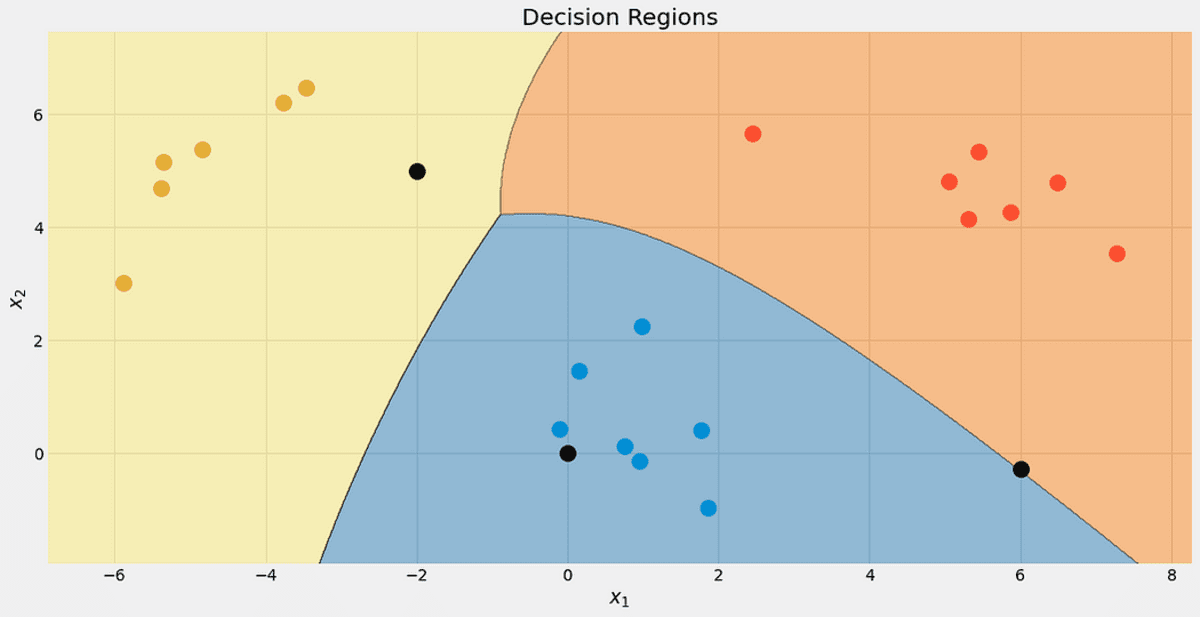
The decision regions with the 3 new points. Image by the Author.

Conclusion

In this article, we have learned how the Gaussian naive Bayes classifier works and gave an intuition on why it was designed that way — it is a direct approach to model the probability of interest. Compare this with Logistic regression: there, the probability is modeled using a linear function with a sigmoid function applied on top of it. It’s still an easy model, but it does not feel as natural as a naive Bayes classifier.

We continued by calculating a few examples and collecting some useful pieces of code on the way. Finally, we have implemented a complete Gaussian naive Bayes classifier in a way that works well with scikit-learn. That means you can use it in pipelines or grid search, for example.

In the end, we did a small sanity check by importing scikit-learns own Gaussian naive Bayes classifier and testing if both, our and scikit-learn’s classifier yield the same result. This test was successful.

 
 
Dr. Robert Kübler is a Data Scientist at METRO.digital and Author at Towards Data Science.

 
Original. Reposted with permission.