We interact with machines on a daily basis – whether it's asking “OK Google, set the alarm for 6 AM” or “Alexa, play my favorite playlist”. But these machines do not understand natural language. So what happens when we talk to a device? It needs to convert the speech i.e. text to numbers for processing the information and learning the context. In this post, you will learn one of the most popular tools to convert the language to numbers using CountVectorizer. Scikit-learn’s CountVectorizer is used to recast and preprocess corpora of text to a token count vector representation. 

Source

How does it work?

Let's take an example of a book title from a popular kids' book to illustrate how CountVectorizer works. 

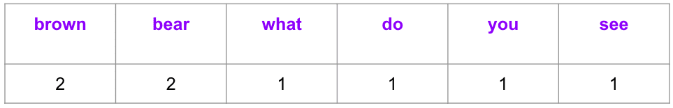
text = ["Brown Bear, Brown Bear, What do you see?"]

There are six unique words in the vector; thus the length of the vector representation is six. The vector represents the frequency of occurrence of each token/word in the text.

Let's add another document to our corpora to witness how the dimension of the resulting matrix increases.

text = ["Brown Bear, Brown Bear, What do you see?", “I love you to the moon and back”]

The CountVectorizer would produce the below output, where the matrix becomes a 2 X 13 from 1 X 6 by adding one more document.

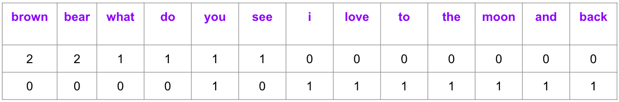
Each column in the matrix represents a unique token (word) in the dictionary formed by a union of all tokens from the corpus of documents, while each row represents a document. The above example has two book titles i.e. documents represented by two rows where each cell contains a value identifying the corresponding word count in the document. As a result of such representation, certain cells have zero value wherever the token is absent in the corresponding document.

Notably, it becomes unmanageable to store huge matrices in memory with the increasing size of the corpora. Thus, CountVectorizer stores them as a sparse matrix, a compressed form of the full-blown matrix discussed above.

Hands-On!

Let's pick the Harry Potter series of eight movies and one Indiana Jones movie for this demo. This would help us understand some important attributes of CountVectorizer.

Start with importing Pandas library and CountVectorizer from Sklearn > feature_extraction > text. 

import pandas as pd
from sklearn.feature_extraction.text import CountVectorizer

Declare the documents as a list of strings.

text = [
    "Harry Potter and the Philosopher's Stone",
    "Harry Potter and the Chamber of Secrets",
    "Harry Potter and the Prisoner of Azkaban",
    "Harry Potter and the Goblet of Fire",
    "Harry Potter and the Order of the Phoenix",
    "Indiana Jones and the Raiders of the Lost Ark",
    "Harry Potter and the Half-Blood Prince",
    "Harry Potter and the Deathly Hallows - Part 1",
    "Harry Potter and the Deathly Hallows - Part 2"
]

Vectorization

Initialize the CountVectorizer object with lowercase=True (default value) to convert all documents/strings into lowercase. Next, call fit_transform and pass the list of documents as an argument followed by adding column and row names to the data frame.

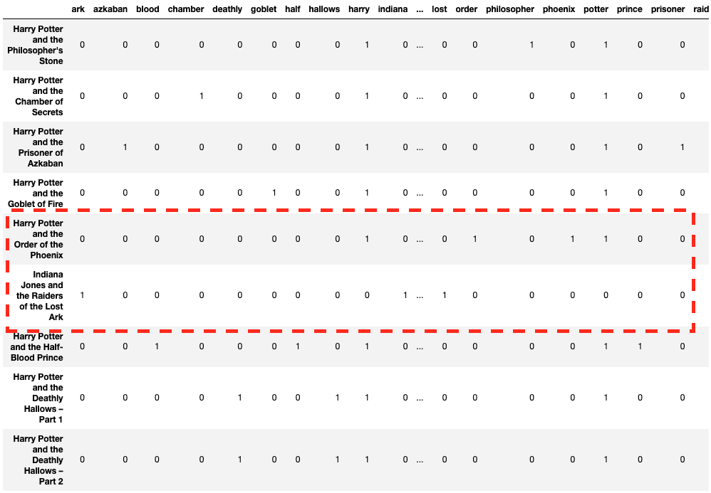
count_vector = CountVectorizer(lowercase = True)
count_vektor = count_vector.fit_transform(text)
count_vektor = count_vektor.toarray()
df = pd.DataFrame(data = count_vektor, columns = count_vector.get_feature_names())
df.index = text
df

Good news! The documents are converted to numbers. But, a close look shows that “Harry Potter and the Order of the Phoenix” is similar to “Indiana Jones and the Raiders of the Lost Ark” as compared to other Harry Potter movies - at least at the first glance.  

You must be wondering if tokens like ‘and’, ‘the’, and ‘of’ add any information to our feature set. That takes us to our next step i.e. removing stop words.

stop_words

Uninformative tokens like ‘and’, ‘the’, and ‘of’ are called stop words. It is important to remove stop words as they impact the document's similarity and unnecessarily expand the column dimension.

Argument ‘stop_words’ removes such preidentified stop words – specifying ‘english’ removes English-specific stop words. You can also explicitly add a list of stop words i.e. stop_words = [‘and’, ‘of’, ‘the’].

count_vector = CountVectorizer(lowercase = True, stop_words =
    'english')
count_vektor = count_vector.fit_transform(text)
count_vektor = count_vektor.toarray()
df = pd.DataFrame(data = count_vektor, columns = count_vector.get_feature_names())
df.index = text
df

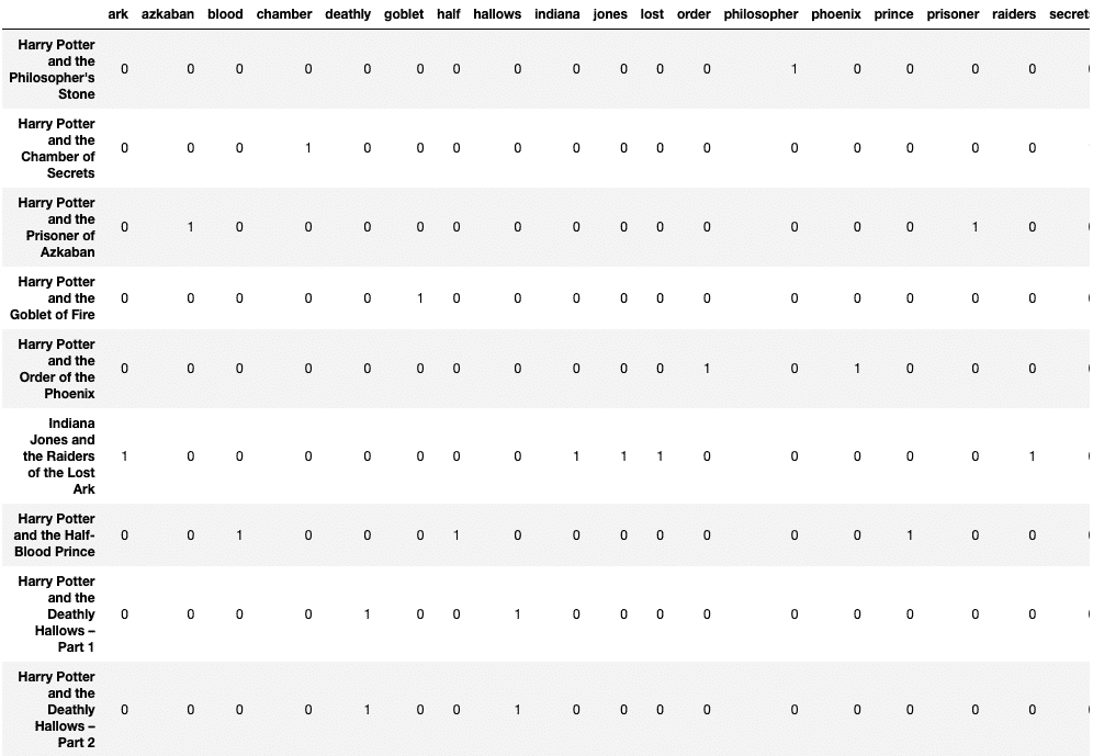
Looks better! Now the row vectors look more meaningful.

max_df

Words like “Harry” and “Potter” aren’t “stop words” but are quite common and add little information to the Count Matrix. Hence, you can add max_df argument to stem repetitive words as features. 

count_vector = CountVectorizer(lowercase = True, max_df = 0.2)
count_vektor = count_vector.fit_transform(text)
count_vektor = count_vektor.toarray()
df = pd.DataFrame(data = count_vektor, columns = count_vector.get_feature_names())
df.index = text
df

Below output demonstrates that stop words as well as “harry” and “potter” are removed from columns:
 

min_df

It is exactly opposite to max_df and signifies the least number of documents (or proportion and percentage) that should have the particular feature.

count_vector = CountVectorizer(lowercase = True, min_df = 2)
count_vektor = count_vector.fit_transform(text)
count_vektor = count_vektor.toarray()
df = pd.DataFrame(data = count_vektor, columns = count_vector.get_feature_names())
df.index = text
df

Here the below columns (words) are present in at least two documents.
 

max_features

It represents the topmost occurring features/words/columns.

count_vector = CountVectorizer(lowercase = True, max_features = 4)
count_vektor = count_vector.fit_transform(text)
count_vektor = count_vektor.toarray()
df = pd.DataFrame(data = count_vektor, columns = count_vector.get_feature_names())
df.index = text
df

Top four commonly occurring words are chosen below.
 

binary

The binary argument replaces all positive occurrences of words by ‘1’ in a document. It signifies the presence or absence of a word or token instead of frequency and is useful in analysis like sentiment or product review.

count_vector = CountVectorizer(lowercase = True, binary = True,
    max_features = 4)
count_vektor = count_vector.fit_transform(text)
count_vektor = count_vektor.toarray()
df = pd.DataFrame(data = count_vektor, columns = count_vector.get_feature_names())
df.index = text
df

Upon comparing with the previous output, the frequency table of the column named “the” is capped to ‘1’ in the result shown below:
 

vocabulary_

It returns the position of columns and is used to map algorithm results to interpretable words.

count_vector = CountVectorizer(lowercase = True)
count_vector.fit_transform(text)
count_vector.vocabulary_

The output of the above code is shown below.

{
    'harry': 10,
    'potter': 19,
    'and': 0,
    'the': 25,
    'philosopher': 17,
    'stone': 24,
    'chamber': 4,
    'of': 14,
    'secrets': 23,
    'prisoner': 21,
    'azkaban': 2,
    'goblet': 7,
    'fire': 6,
    'order': 15,
    'phoenix': 18,
    'indiana': 11,
    'jones': 12,
    'raiders': 22,
    'lost': 13,
    'ark': 1,
    'half': 8,
    'blood': 3,
    'prince': 20,
    'deathly': 5,
    'hallows': 9,
    'part': 16
}

Summary

The tutorial discussed the importance of pre-processing text aka vectorizing it as an input into machine learning algorithms. The post also demonstrated sklearn’s implementation of CountVectorizer with various input parameters on a small set of documents. 

 
 
Vidhi Chugh is an award-winning AI/ML innovation leader and an AI Ethicist. She works at the intersection of data science, product, and research to deliver business value and insights. She is an advocate for data-centric science and a leading expert in data governance with a vision to build trustworthy AI solutions.